Detecting Election Result Irregularities in Kaduna(Nigeria) Using Geospatial Analysis.

During my Internship at HNG Tech, I performed geoanalytics on election results recorded in Kaduna, a state in Nigeria. The goal was to help the data analytics team uncover potential influences in the 2023 election results in Nigeria. I volunteered to analyse the dataset on election results from kaduna. I thoroughly enjoyed every second of this project and I wanted to present my analytics process and what I discovered.
In this blog I will discuss the steps I took to prepare the data for analysis and the steps I took to build an interactive map to assist stakeholders investigate the anomalies detected from the statistical analysis.
Executive Summary
Based on the results of my analysis, election officials or relevant stakeholders should start looking into some severe anomalies detected in the 2023 election results from Kaduna, especialy vote entires for NNPP at the polling units in Kaduna with the following codes;
PU_Code: 18–15–05–032
PU_Code: 18–21–05–001
PU_Code: 18–21–02–009It is also interesting to note that all three polling units recorded the exact same number of votes for NNPP. To assist the team with investigations I created the Election Anomaly Inspector application using the results of the analysis.
Prerequisites
To be able to follow along you will need;
- A basic understanding of Python. See this resource
- Ability to set up Python environment for data analysis. see this resource
- A basic understanding of Google Earth Engine. See this resource
- Familiarity with libraries like geopy, numpy, pandas, and Scikit-learn.
Task Description
pinpoint polling units where the voting results significantly deviate from their neighbours, indicating potential irregularities or influences.
I broke down tasks into these subtasks:
- Prepare dataset for analysis
- Identify Neighbouring Polling Units
- Calculate Outlier Scores for each party
- Sort and Report on the Data Using Visualisation.
Preparing Dataset
For the election outlier detection task, I focused on election results from Kaduna, a state in Nigeria. The given dataset contained information about the polling units, the votes each party received, and the election results. The dataset is in CSV format.
I checked the data for `Null` values and spot-checked for longitude and latitude coordinate columns.
import pandas as pd

# read csv file
df = pd.read_csv('KADUNA_crosschecked.csv')
# inspect columns and check for null values
df.isnull().sum()
I got the output below indicating no null values in all the columns.
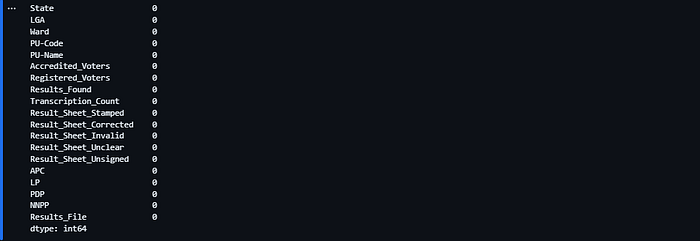
and I also noticed there are no coordinates to work with, so we will create one in the coming section.
For our analysis these columns will not be relevant: Results_File , Transcription_Count , Result_Sheet_Stamped , Result_Sheet_Corrected , Result_Sheet_Unclear , Result_Sheet_Invalid , Results_Found , Registered_Voters and Acredited_Voters . We will need to drop them.
columns_to_drop = ['Accredited_Voters', 'Registered_Voters',
                   'Results_Found', 'Transcription_Count',
                   'Result_Sheet_Stamped', 'Result_Sheet_Corrected',
                   'Result_Sheet_Invalid', 'Result_Sheet_Unclear',
                   'Result_Sheet_Unsigned', 'Results_File'
                    ]
for column in columns_to_drop:
    df.drop(column, axis=1, inplace=True)
Extracting Longitude and Latitude Values
For the geocoding procedure, I chose the geopy package. The geopy library makes it easy for developers to locate the coordinates of addresses, cities, countries, and landmarks across the globe using third-party geocoders like Google, Bing, HERE, QGIS, US Census Bureau, and Esri.
With the help of Google Geocoding API, I geocoded the dataset using a Python script I wrote.
Step One: Retrieve Precise Location of Polling Units
import pandas as pd

import pandas as pd

def create_location(row: pd.Series) -> str:
    # Extract LGA and Ward from the row
    LGA = row['LGA']
    Ward = row['Ward']
    PU_Name = row['PU-Name']

    # Combine LGA and Ward into a location string
    location = f"{LGA}, {Ward}, {PU_Name}, Kaduna, Nigeria"
    return location

# Testing the create_location function
df_copy = df.copy()
df_copy['Location'] = df.apply(create_location, axis=1)
df_copy['Location'][0]
Testing the function should return the output below:
'BIRNIN GWARI, MAGAJIN GARI I, PRY. SCH. SHITU, Kaduna, Nigeria'From the above output string, we can see that the script correctly combines the LGA , Ward, and PU-Namecolumns to create a more precise location string which ispassed to a create_geocode() function we will soon write.
Step Two: Get Geocode Based on Precise Location
I wrote another function that uses the location string for each polling unit to retrieve the longitude and latitudes.
from geopy.geocoders import GoogleV3
from geopy.extra.rate_limiter import RateLimiter
import os
from dotenv import load_dotenv #for loading .env file which has My API key

load_dotenv()
api_key = os.getenv('GMAP')

# create geocoder instance and set rate limits
geolocator = GoogleV3(api_key=api_key)
geocode = RateLimiter(geolocator.geocode, min_delay_seconds=1)

# create geocode function
def create_geocode(location: str) -> str:
    """Creates a geocode based on a given location
    Args:
        location(str)
    Return:
        str: geocode
    """
    try:
        return geocode(location)
    except:
        return None
The code creates a geocode using the Google Maps API. To be able to access the Google map API you need to get the API credential .
After getting the API credential, create a .env file and add this variable GMAP=<your_api_credential> we then used os.getenv('GMAP') to load the API key from the.env file. We then instantiated the GoogleV3 geocoder instance using the API key and added a rate limiter to ensure that geocoding requests do not exceed one request per second.
Finally, we defined a create_geocode()function to geocode a given location string using the GoogleV3 geocoder. If the geocoding operation fails, the function returns None.
In the next steps, we will use the create_geocode() function to update our dataset with the geo-location data.
Putting it All Together
I used the create_location()function to create a Location column in our dataset. I then used the create_geocode() function to retrieve all geocode.
After getting the geocode, I extracted the longitude and latitude columns.
# create Location Column
df['Location'] = df.apply(create_location, axis=1)

# create Geocode
df['geocode'] = df['Location'].apply(create_geocode)

# extract longitude and Latitude from Geocode
df['latitude'] = df['geocode'].apply(lambda x: x.latitude if x else None)
df['longitude'] = df['geocode'].apply(lambda x: x.longitude if x else None)

# Save output in a file
df.to_csv('KADUNA_geocoded_data.csv', index=False)
Identifying Neighbouring Polling Units
To identify neighbouring polling units, let’s use a simple heuristic:
Polling units are considered neighbours if the distance between them is 1 kilometre
To compare the distance between the polling units we need to know the actual distances between all the polling units.
We will then compare the distances to the 1-kilometre rule of thumb to identify the neighbouring polling units.
I Followed These steps:
1. Use the Harversine Formula to calculate the distance between polling units.
2. Check for neighbours based on the rule of thumb, using an identify_neighbor()function.
1. Find The Harvensine Distance Between Polling Units in Kaduna
from geopy.distance import geodesic

# define function to calculate distance

def haversine_distance(coord1, coord2):
    return geodesic(coord1, coord2).km
The code above defines a function for calculating the distance between two points using the geodesic() function provided by the geopy library. It is based on the Haversine Formula and it accepts two coordinates as arguments which will be used to find the distance.
In the next step, we will define an identify_neighbor()function to find neighbouring polling units.
2. Find Neighboring Polling Units
def identify_neighbor(df, radius_km=1):

    # Extract coordinates
    coords = df[['latitude', 'longitude']].to_numpy()

    # Create KD-Tree
    tree = cKDTree(coords)

    neighbors = []
    for idx, coord in enumerate(coords):
        # Find initial candidates within a bounding box of approximately 1 km
        indices = tree.query_ball_point(coord, radius_km / 6371.0)
        neighbor_indices = [i for i in indices if i != idx]

        # Filter candidates using the Haversine function
        true_neighbors = [
            i for i in neighbor_indices if haversine_distance(coord,
                                                     coords[i]) <= radius_km
        ]
        neighbors.append(true_neighbors)

    # Add neighbors to DataFrame
    df['neighbors'] = neighbors
    return df

neighbors_df = identify_neighbor(geocoded_df, radius_km=1)
neighbors_df.to_csv('KADUNA_with_neighbors.csv')
The identify_neighbor()function accepts a dataframe and a radius in kilometers, it then extracts coordniate information and finds the initial candidates for comparison using the harvesine_distance()
Putting it all together
I saved the output of the function in a csv for further analysis.
import pandas as pd

# read geocoded data
geocoded_df = pd.read_csv('KADUNA_geocoded_data.csv')

# identify neighbours
neighbors_df = identify_neighbor(geocoded_df, radius_km=1)

# save data to a csv file
neighbors_df.to_csv('KADUNA_geocoded_with_neighbors.csv')
At this point, I had enough data points to proceed with the next key part of the task; finding outlier scores
Calculate Outlier Scores for each party
For each polling unit(PU_Name), I will compare the votes for each party with those of its neighbouring units.
There are four political parties to consider for each polling unit;
- APC
- LP
- PDP
- NNPP
I calculated an outlier score for each party based on the deviation of votes from neighbouring units.
I recorded the outlier scores along with the respective parties and neighbouring units.
I followed these steps:
1. Choosing The Appropriate Statistical Method
The choice of the appropriate statistical method for calculating outlier scores depends on several factors including the distribution of the data, the type of data, and the context of the analysis.
To help me decide on the right statistical approach to calculating outlier scores, I needed to understand the type of distribution the votes have per political party.
I used Q-Q plots to examine the distribution and performed the Shapiro-Wilk test to determine normality in the distribution of votes per political party.
I put all this in a check_normality() function to perform the checks for normality on the distribution.
import matplotlib.pyplot as plt
from scipy.stats import shapiro
import statsmodels.api as sm

def check_normality(dataframe, parties):
    num_parties = len(parties)
    num_cols = 2
    num_rows = (num_parties + 1) // num_cols

    fig, axs = plt.subplots(num_rows, num_cols, figsize=(12, 6 * num_rows))
    axs = axs.flatten()

    for i, party in enumerate(parties):
        votes = dataframe[party].dropna()

        print(f"Checking distribution for {party} votes")

        # Q-Q Plot
        sm.qqplot(votes, line='45', ax=axs[i])
        axs[i].set_title(f'Q-Q Plot of {party} Votes')

        # Shapiro-Wilk Test
        shapiro_test = shapiro(votes)
        print(f'Shapiro-Wilk Test p-value for {party}:', shapiro_test.pvalue)
        if shapiro_test.pvalue > 0.05:
            print(f"The distribution of {party} votes is likely normal.")
        else:
            print(f"The distribution of {party} votes is likely not normal.")
        print("\n")

    # Hide any unused subplots
    for j in range(i + 1, num_rows * num_cols):
        fig.delaxes(axs[j])

    plt.tight_layout()
    plt.show()
Performing the Check
# Load the CSV file into a DataFrame
normal_dist_df = neighbors_df

# List of political parties
parties = ['APC', 'LP', 'PDP', 'NNPP']

# Check normality for each party
check_normality(df, parties)
Results
Checking distribution for APC votes
Shapiro-Wilk Test p-value for APC: 2.6345688074106287e-59
The distribution of APC votes is likely not normal.


Checking distribution for LP votes
Shapiro-Wilk Test p-value for LP: 3.4330261622692515e-78
The distribution of LP votes is likely not normal.


Checking distribution for PDP votes
Shapiro-Wilk Test p-value for PDP: 2.1798802282225605e-48
The distribution of PDP votes is likely not normal.


Checking distribution for NNPP votes
Shapiro-Wilk Test p-value for NNPP: 1.0787169297523082e-78
The distribution of NNPP votes is likely not normal.
Q-Q plots
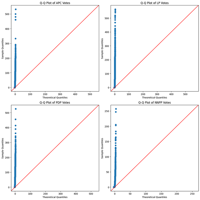
As can be seen, the distribution of the voting pattern for all four parties does not follow the normal distribution and so statistical methods like the basic Z-score approach will not be particularly effective in finding the outliers. This is because the approach assumes a normally distributed data contrary to what we discovered.
I settled on using the Local Outlier Factor Method(LOF) to calculate the outlier scores of the political parties in each polling unit. The Local Outlier Factor (LOF) method provided by scikit-learn is an unsupervised Machine Learning anomaly detection technique that identifies outliers by comparing the concentration of data points within a specific area in a given dataset.
In analyzing voting patterns, LOF is useful because of its ability to handle multivariate data and capture complex interactions between votes for different parties. By focusing on local variations, LOF can uncover easy to miss irregularities in specific polling units, providing a more nuanced understanding of outlier voting behaviours. I am confident that this capability makes LOF a suitable and robust choice for this outlier detection task.
Calcuating LOF Scores
import pandas as pd
from sklearn.preprocessing import StandardScaler
from sklearn.neighbors import LocalOutlierFactor
import numpy as np

# Load election data
election_data = pd.read_csv('KADUNA_with_neighbors.csv')

# Define party columns
party_columns = ['APC', 'LP', 'PDP', 'NNPP']

def calculate_lof_for_each_party(data, party_columns):
    scaler = StandardScaler()
    for party in party_columns:
        # Apply a logarithmic transformation to reduce skewness
        data[f'{party}_log'] = np.log1p(data[party])

        # Standardize the log-transformed data
        normalized_column = f'{party}_norm'
        lof_column = f'{party}_lof_score'
        data[normalized_column] = scaler.fit_transform(data[[f'{party}_log']])

        # Adjust LOF parameters based on experimentation
        clf = LocalOutlierFactor(n_neighbors=15, contamination=0.05)

        # Fit the model and predict outliers
        data[f'{party}_outlier_flag'] = clf.fit_predict(data[
                                                        [normalized_column]
                                                         ])

        # Assign LOF scores
        data[lof_column] = clf.negative_outlier_factor_

    return data

# Calculate LOF scores for each party
election_data = calculate_lof_for_each_party(election_data, party_columns)
Displaying results
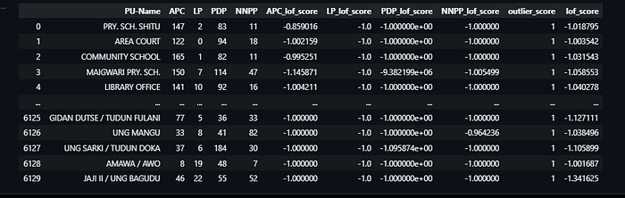
from IPython.display import display

columns_to_display = election_data[['PU-Name', 'APC',
                                    'LP', 'PDP', 'NNPP',
                                    'APC_lof_score',
                                    'LP_lof_score','PDP_lof_score',
                                    'NNPP_lof_score',
                                    'outlier_score', 'lof_score']]
display(columns_to_display)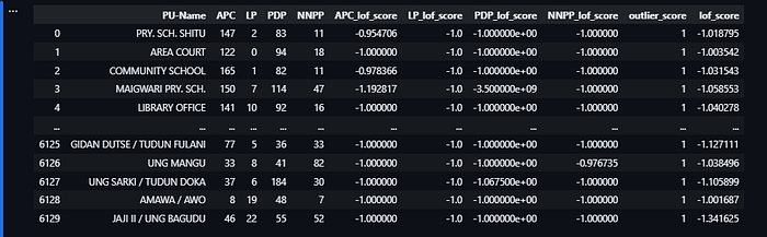
Interpreting the Scores
The Local Outlier Factor scores <party_name>_lof_score represents real-valued floats that indicate how much some votes for a party in a polling unit deviate from its local neighbourhood density.
- LOF Score < 1: Indicates that the votes observed in a polling unit are in a relatively dense region and are similar to its neighbours.
- LOF Score > 1: Indicates that the votes observed are in a less dense region and may be considered an outlier compared to its neighbours.
<party_name>_lof_score column represents outlier scores for a party.
In the next steps, I will sort and report on the outlier scores observed on the election results to determine the regions with the highest outliers.
Sorting and Reporting on Findings
The goal of this section is to sort the dataset by the outlier scores for each party to identify the most significant outliers. I will Highlight the top 3 outliers and their closest polling units.
Sorting Party LOF Scores
Let’s define a sort_party_lof function to sort data for multiple parties based on their individual Local Outlier Factor (LOF) scores.
import pandas as pd

def sort_party_lof(dataframe, party_name, lof_score_column):
    # Select relevant columns
    columns_to_select = ['State',
                         'LGA',
                         party_name,
                         'latitude',
                         'longitude',
                         'neighbors',
                         'geocode',
                         lof_score_column]

    existing_columns = [col for col in columns_to_select
                        if col in dataframe.columns]
    # Select the relevant columns from the DataFrame
    selected_data = dataframe[existing_columns]
    # Sort the selected data by the LOF score column in ascending order
    sorted_data = selected_data.sort_values(by=lof_score_column,
                                            ascending=True)
    return sorted_data

party_names = ['APC', 'PDP', 'NNPP', 'LP']

sorted_scores = []

for party_name in party_names:
    sorted_party = f"sorted_{party_name}"
    sorted_scores.append(sort_party_lof(scores_df,
                          party_name, f"{party_name}_lof_score"))
The sort_party_lof accepts a dataframe, the name of the party and the name of the lof score column to retrieve. The function retrieves only the columns listed, it then creates a dataframe object and sorts the data by the lof score column in ascending order.
I called the sort_party_lof function in a for loop to retrieve the sorted LOF scores for all four political parties. All the sorted dataframe objects are stored in the sorted_scores list for later analysis.
Top Outlier Votes Recorded for APC Party.
we can access the sorted lof_score dataframe for APC by checking the first element of the sorted_scores list.
sorted_apc = sorted_scores[0]
sorted_apc.head(3)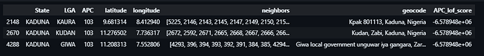
The LOF Score of -6.578948e+06 for APC represents an extremely high deviation from the distribution of votes. The same observation was made in the top 3 LOF scores of LP, PDP and NNPP.
You can repeat the process above to see the top 3 scores for the remaining parties.
Reasons that may account for these extremely high outliers may include the following:
- A problem with my approach to calculating the LOF score: To rule out this possibility I cross-checked my steps, applied normalisation techniques, and experimented with different parameters for the
LocalOutlierFactor(n_neighbors=n, contamination=n)class. Additionally, looking at the LOF scores data, in general, reveals several instances where normal distributions were observed.
2. A problem with the data entry: the anomalies observed most likely point to data-specific issues that prompt further contextual investigation. For instance, in all the top 3 outlier scores, the number of votes is the same for 3 different polling units with different locations resulting in the same values for LOF scores.
Visualisation
Preparing Dataset for visualisation
Currently, our sorted_scores variable holds the dataframes for the top three outlier scores for each party. we need to export them as csv files for later analysis.
Export CSV Sample Files
# export file for APC
sorted_apc = sorted_scores[0]
sorted_apc.head(3).to_csv('outliers_APC.csv')

# export file for PDP
sorted_pdp = sorted_scores[1]
sorted_pdp.head(3).to_csv('outliers_PDP.csv')

# export file for NNPP
sorted_nnpp = sorted_scores[2]
sorted_nnpp.head(3).to_csv('outliers_NNPP.csv')

# export file for NNPP
sorted_lp = sorted_scores[3]
sorted_lp.head(3).to_csv('outliers_LP.csv')
The neighbors column contains index values we can use to find more information on each neighboring polling unit. Let’s retrieve the LOF score for each neighbor in the list of neighbors for each sample file.
def retrieve_neighbor_insights(source,  lof_column_name, sample=None,):
    # Step 1: Load the source DataFrame
    source_df = pd.read_csv(source)

    # Step 2: Check if a sample DataFrame is provided and load it
    if sample:
        sample_df = pd.read_csv(sample)
    else:
        sample_df = source_df.copy()

    # Prepare the 'neighbors' column in both DataFrames
    source_df['neighbors'] = source_df['neighbors'].apply(lambda x: eval(x))
    sample_df['neighbors'] = sample_df['neighbors'].apply(lambda x: eval(x))

    sample_df['neighbor_score'] = [[] for _ in range(len(sample_df))]

    # Iterate over each row in the sample DataFrame
    for index, row in sample_df.iterrows():
        for neighbor_index in row['neighbors']:
            if neighbor_index in source_df.index:
                # Retrieve the LOF score for that neighbor
                neighbor_lof_score = source_df.loc[
                                                    neighbor_index,
                                                    lof_column_name
                                                   ]

                sample_df.at[index, 'neighbor_score'].append(float(neighbor_lof_score))

    # Return the updated sample DataFrame
    return sample_df
Let’s run the retrieve_neighbor_insights() function in a for loop to find the lof scores for neighboring polling units.
political_parties = ['APC', 'PDP', 'NNPP', 'LP']

for party in political_parties:
    # Retrieve neighbor insights for each party
    outliers_insight = retrieve_neighbor_insights('KADUNA_outlier_scores.csv',
                                                   f'{party}_lof_score',
                                                   f'outliers_{party}.csv')

    # Check if the DataFrame has an unnamed column and rename it
    if 'Unnamed: 0' in outliers_insight.columns:
        outliers_insight.rename(columns={'Unnamed: 0': 'index'},
                                inplace=True)
    else:
        # Reset the index to create a new 'index' column
        outliers_insight.reset_index(inplace=True)
        outliers_insight.rename(columns={'index': 'index'}, inplace=True)

    # Save the DataFrame to a CSV without adding index column
    outliers_insight.to_csv(f'outliers_insight_{party}.csv', index=False)
The code above creates the following csv files which will be used for our visualisation:
outliers_insight_APC.csvoutliers_insight_PDP.csvoutliers_insight_NNPP.csvoutliers_insight_LP.csv
Ranking Severity of Election Vote Anomalies by Party
First, let’s observe the ranking of LOF scores for all parties using the code below.
import pandas as pd
import matplotlib.pyplot as plt
import numpy as np


filenames = ['outliers_insight_PDP.csv',
             'outliers_insight_APC.csv',
             'outliers_insight_LP.csv',
             'outliers_insight_NNPP.csv']
party_names = ['PDP', 'APC', 'LP', 'NNPP']
scores = {}

for file_name, party_name in zip(filenames, party_names):
    df = pd.read_csv(file_name)
    score_column = f"{party_name}_lof_score"
    scores[party_name] = df[score_column].head(3).tolist()

def visualize_scores(scores):

    parties = list(scores.keys())
    data = np.array([scores[party] for party in parties])


    fig, ax = plt.subplots()
    cax = ax.matshow(data, cmap="viridis")


    ax.set_xticklabels([''] + ['Top 1st',
                                'Top 2nd',
                                'Top 3rd'
                               ], minor=False)
    ax.set_yticklabels([''] + parties, minor=False)


    for (i, j), val in np.ndenumerate(data):
        ax.text(j, i, f"{val:.2f}",
                ha='center',
                va='center',
                 color="white")

    plt.colorbar(cax)
    plt.show()

visualize_scores(scores)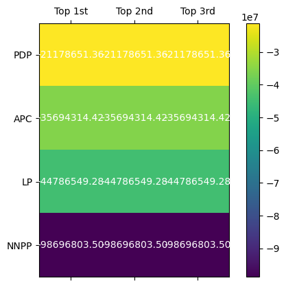
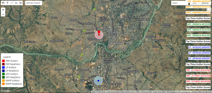
Visualising Election Irregularity On Interactive Map.
For this visualization, Let’s build an interactive map application that can help election officials and stakeholders investigate the election anomalies in Kaduna. The stakeholders should be able to see the polling units with the highest anomalies and their neighbouring polling units.
Requirements
1. Ability to see the top 3 outliers for each party on the map
2. Ability to spot the neighboring polling units and observe the outlier scores of polling units in the vicinity.
3. Ability to see at a high level the spread of anomalies.
I wrote this javascript that runs in the google earth engine console to visualise the location of the outlier scores.
Conclusion and Recommendations
During the analysis, I discovered these key anomalies in the votes recorded in some polling units across all four political parties.
- NNPP had the most severe cases of deviation in voting distributions
- In all the top three outlier scores for each party, votes across different polling units were the same.
- Further field Investigations needs to be done to understand these anomalies in order to confirm or rule out possible influences in election results in Kaduna. A good place to start is with the Election Anomaly Inspector